Collective motion describes the motion of a group. These members of the group are referred to as agents. Examples in nature of collective motion are schools of fish, flocks of birds, and colonies of bacteria.
In this research with Professor Andy Borum, we analyze collective motion through the lens of optimal control theory. We treat variables such as agent velocity or agent angle as control inputs to optimize our cost function. As we increase the number of agents in our system, we can incorporate synchronization of motion through coupling parameters. We explore the optimal trajectories with this setup.
Example Setup
Visually, each agent’s motion in 2D can be described with 3 variables shown below.
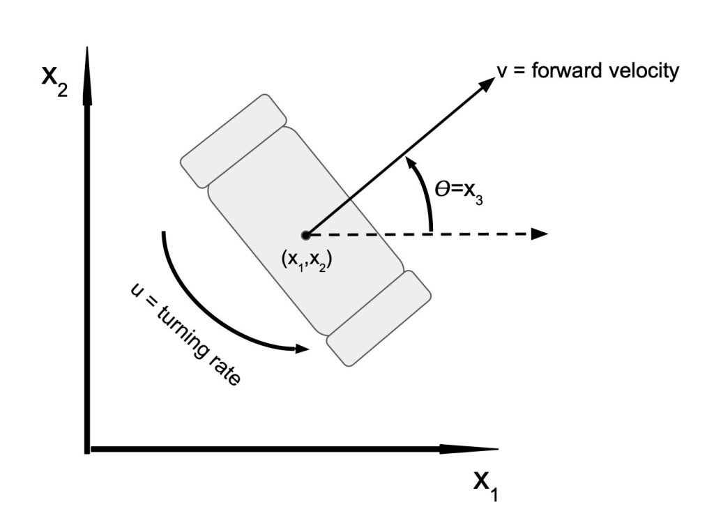
With these variables, our optimal control problem looks like the following.
$$ \begin{aligned} \min_{x,u} \quad & \int_{t_0}^{t_f} g(x(t),u(t))\,dt \\ \text{subject to} \quad & \dot{x}(t)=f(x(t),u(t)), \\ & x(0)=x_0,\quad x(t_f)=x_f \end{aligned} $$
For us, we impose an ice skate constraint, meaning the velocity of the robot is only in the heading direction (zero velocity in the perpendicular direction). This makes \(\dot{x}\) look like the case below.
$$ \begin{align} \dot{x} &= \begin{pmatrix} v\cos(\theta)\\ v\sin(\theta)\\ u \end{pmatrix} \end{align} $$